
Advocates for the reformation of our national educational policies often call for more competition in our schools because of the belief that market forces will lead to greater efficiency. However, just how should this competition be defined? How do certain geographic and demographic variables affect the establishment of a national policy? Researchers from Saginaw Valley State, Pittsburg State and Mississippi State set out to apply GIS tools to the development of a school competition index in the state of Mississippi to see if these questions could be resolved. In sum, the authors found that higher levels of competition from private schools significantly increased public school productivity. Let’s see how they got there.
 Public and private schools in Mississippi, and private schools in neighboring states.
 School Competition Index for Starkville High School in Starkville, MS which is also home to Mississippi State University.
In their preliminary research and literature review, the authors gave consideration to the two overriding philosophies in educational reform: high-stakes tests and market-type reforms. The former’s goal is to increase measured achievement levels of students; while the latter allows students to attend public schools in their districts, or to attend private schools of their choice with discount vouchers to absorb some of the cost. As there have been mixed findings on the benefits of inner-school competition and performance, the results are too conflicting to draw any generalizations, hence the need for this study.
To examine the relationship between competition and technical efficiency, the study included a two-pronged approach, the first of which explores school outputs based on a number of variables. The estimates of technical efficiency were then used as dependent variables in a regression analysis with school performance. It was found that competition from private schools extended into neighboring states as well, including Alabama, Arkansas, Tennessee and Louisiana. The majority of data was obtained from the Mississippi Department of Education, and most variables came from the Mississippi Report Card, an annual accounting of school statistics.
There were numerous interesting findings in this study based on the variables provided by the state of Mississippi. The Primary School model indicated a positive correlation between the percentage of students receiving free lunches and inefficiency. In the High School sample, female principals were commonly associated with inefficiency as well as with public schools. Student’s race was not found to be a significant factor in any model, though socioeconomic status was, as indicated by the free lunch result. Another interesting finding that I was shocked to see was that human capital, in the form of teaching experience and educational attainment, had insignificant impact on the Primary School model; however in the High School model, these factors were very significant. This led the authors to try and conclude why experience or academic pedigree is not impactful at younger ages. Is it because younger students don’t benefit from the structure often acquired through graduate education or the development of classroom practice from seasoned teachers? This study highlighted key elements in one state’s performance, but also brought up many more questions that may be valuable in shaping our nation’s educational system, and thus the future of our country.
Justin Harmon
Staff Writer
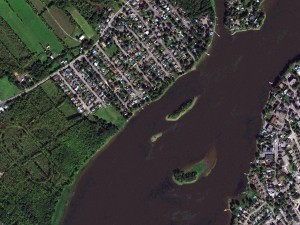
 1.5-meter SPOT 6 natural color images collected over Royal Montreal Golf Course, Quebec and the surrounding areas on September 17, 2013. If you would like to see this golf course in Pléiades 1 50-cm resolution as a comparison, please click here. © CNES 2012, Distribution Airbus Defense and Space / Spot Image S.A., France, all rights reserved
 This map of SPOTMap1.5 coverage shows the regions that have been released as well as those currently in production. An Apollo Mapping representative can provide more details on the specific year ranges used in each mosaic.
 This map of SPOTMap2.5 coverage has been color coded to show the collection year which makes up the majority of each mosaic as well as those markets that were added in the final month of production (i.e. August 2013). An Apollo Mapping representative can provide more details on the specific year ranges used in each mosaic.
In this monthly article, we provide details on updates to Airbus Defense and Space GEO’s SPOTMaps product. SPOTMaps is an orthorectified 2.5-meter (m) and now 1.5-m natural color imagery layer with coverage over more than 100 countries–totaling an impressive 108 million plus square kilometers (sq km). For projects requiring a value-priced basemap better than what 15-m Landsat can offer, there is no other choice than SPOTMaps.
SPOTMaps Product Updates–June 2014
- 22 million sq km of SPOTMap1.5 coverage is to be released in 2014 alone!
- These countries are currently in production and will be added to the SPOTMaps1.5 database soon:
- Iran (part of the country)
- Iraq (part of the country)
- New Zealand
- Niger (part of the country)
- Oman
- Saudi Arabia (part of the country)
- South Africa (most of the country)
- United Arab Emirates
- Yemen
- Production of SPOTMaps2.5 is complete now that SPOTMaps1.5 are being released.
Key Product Specifications
- SPOTMaps1.5
- Resolution: 1.5-m
- Spectral Bands: true natural color (RGB)
- Horizontal Accuracy: 6 to 10-m CE90 (circular error 90%)
- Projection/Datum: UTM WGS84
- Source Data: SPOT6/7 satellite imagery
- File Format: GeoTIFF
- SPOTMaps2.5
- Resolution: 2.5-m
- Spectral Bands: simulated natural color (RGB)
- Horizontal Accuracy: 10 to 15-m RMSE (root mean square error)
- Projection/Datum: UTM WGS84
- Source Data: SPOT5 satellite imagery
- File Format: GeoTIFF
For those who have never worked with SPOTMaps, below is a summary of key product specifications of the 1.5-m and 2.5-m versions as well as product differentiators.
Product Differentiators
- Recent and ready for immediate delivery and integration with your GIS
- Seamless, orthorectified coverage across countries and entire regions in 1.5-m and 2.5-m resolution
- Suitable for work up to 1:10,000 scale
- Custom product framing with minimum orders of ~100 sq km
- Product series is updated nearly every month
- Source data can be delivered with all SPOTMaps mosaics
- Volume and academic discounts are offered
- Multi-user licenses are available
If you would like pricing details and/or additional product details, such as date ranges and accuracy specifications, please let us know at sales@apollomapping.com or (303) 993-3863.
Do you need high-resolution satellite imagery collected at nighttime over nearly any location on the planet?
 A chart showing the times of the year (with respect to latitude) that nighttime imaging is possible with EROS B.

 Previews of ~70-cm EROS B imagery collected during the night over Dallas-Fort Worth Airport on September 14, 2008. (Images Courtesy: ImageSat International)
If so, Apollo Mapping has a solution for you! Partnering with ImageSat International, the owner and operator of the satellites EROS A and EROS B, we are able to provide you with custom nighttime collections of ~70-cm panchromatic imagery over areas as small as 50 square kilometers. As an added bonus, the price for this nighttime imagery is still below what you would pay for the minimum collection of color, high-resolution, daytime imagery.
We have tasked EROS B on multiple occasions and have been impressed with the turnaround time and high-quality panchromatic imagery it can deliver. While many people shy away from black and white only data, when it comes to nighttime imagery, there is little to no difference between black and white and color data. Further, by collecting only panchromatic data, EROS B can maximize collection capacity so you receive tasked imagery quicker.
Key Specifications of EROS B
- Launch Date – April 25, 2006
- Spectral Bands – panchromatic only
- Resolution – 70 centimeter (varies with orbital height, off-nadir angle and imaging mode)
- Revisit Time–~3.5 days (varies with latitude and off-nadir angle)
- Swath Width – 7 km (varies with orbital height and off-nadir angle)
- Bit Depth – 10-bits
- Orbit Height – 520 km (varies about this average)
For more information on this new nighttime, high-resolution tasking service, please visit our website or contact the Apollo Mapping sales team at (303) 993-3863 or sales@apollomapping.com.
We are pleased to announce that sales of the much anticipated WorldDEMTM produced by Airbus Defense and Space are under way! For the past three years, Airbus’ twin high-resolution radar satellites, TerraSar-X and TanDEM-X, have imaged the entire land surface of our planet multiple times to create the first ever global 12-meter (m) elevation model. The WorldDEM is ideal for all mapping projects requiring accurate elevation models including orthorectification, floodplain determination, mineral exploration and hydrocarbon development.
 A comparison of 30-m SRTM and 12-m WorldDEMTM elevation data over Arkansas, USA.
WorldDEM Specifications
The key product specifications of Airbus’ WorldDEM are as follows:
- Resolution: 12-m
- Coverage: entire landmass of the Earth, ~150 million square kilometers (sq km)
- Absolute Vertical Accuracy: < 4-m Linear Error 90% (LE90)
- Relative Vertical Accuracy: < 2-m LE90 (slopes ≤ 20%), < 4-m LE90 (slopes > 20%)
- Absolute Horizontal Accuracy: < 10-m Circular Error 90% (CE90)
- Vintage: all data collected within 3 years
- Source: interferometry from synthetic aperture radar (SAR) satellites TerraSAR-X & TanDEM-X
- Minimum Order: 500 sq km per polygon
- File Format: GeoTIFF
- Projection: geographic WGS84 (EGM2008, vertical datum), meter vertical unit
- Product Line Options:
- WorldDEMcore–unedited digital surface model (DSM), includes spikes, wells and voids
- WorldDEM–a DSM with removal of artifacts and water body flattening
- WorldDEM DTM–artifacts and surface features removed, i.e. a digital terrain model (DTM)
WorldDEM Coverage and Pricing
WorldDEM data has a 500 sq km minimum order size with a 10-km width requirement. Prices for two of the product lines have been set:
- WorldDEMcore–$10.80 per sq km
- WorldDEMTM–$13.50 per sq km
 A coverage map of the one-degree cells that are currently ready for production; all of these cells are in North America and Australia so the map views are limited to these areas. The cells on this map are either red (i.e. pre-production phase) or yellow (ready for production). Areas that are ready for production will take approximately four (WorldDEMcore) to eight weeks (WorldDEMTM) to deliver once an order is placed.
Currently, there are portions of the United States, Canada and Australia that are ready for production. In the coming months, the rest of the world will be released. For the estimated release dates of regions not currently ready for production, please email the Apollo Mapping team at sales@apollomapping.com.
WorldDEM Samples
You can download three 12-m WorldDEMTM samples here:
- Buraydah, Saudi Arabia–desert with agriculture present; 576 m to 737 m
- Mjosa Lake, Norway–hilly terrain with large water bodies; 100 m to 840 m
- Wagga Wagga, Australia–forest and urban with many water bodies; 137 m to 922 m
For more information about 12-m WorldDEM data, please send us an email at sales@apollomapping.com.
In last month’s edition of the Geospatial Frequently Asked Question (G-FAQ), we started our two-part discussion on spatial topology in Esri’s ArcGIS. Specifically, we looked at the basics with an exploration of arc-node topology, the types of topology that can be enforced and then several files, i.e. ArcINFO coverages and geodatabases, that can maintain it. In the July edition of the G-FAQ, we wrap up this discussion with a focus on why spatial topology was created as well as the ‘topology’ of shapefiles.
As a quick reminder, this two-part G-FAQ series on spatial topology focuses on three core questions:
What is spatial topology, why is it important and how is it maintained in GIS? What are example files types that are topological in Esri’s ArcGIS? Do shapefiles have topology?
In last month’s G-FAQ, we learned that spatial topology is predicated on an arc-node data structure. Vector files have three basic formats, i.e. points, lines and polygons, which are constructed with nodes, arcs and vertices. The more complex a shape is, the more nodes, arcs and vertices it will have. The spatial topology relationships between the various arcs and nodes in a single vector file are stored in ‘lists’ that ArcGIS can access and interpret. In the case of ArcINFO coverage files, these lists are explicit tables; while for the other most popular file with explicit topology, i.e. geodatabases, they are stored as a set of rules.
Why Was Spatial Topology Created?
Spatial topology is a way to define the geographic relationships between various vector layers in an alternate (and complimentary) fashion to coordinates, such as latitude and longitude. From the research I completed for this G-FAQ series, it appears that topology has been a part of commercially available GIS software from the start. As such, you might ask yourself why this is the case, so let’s try to answer that question.
In order to answer why topology was created, we need to put ourselves in the proper mindset of 1980’s computer technology. These were the days of huge desktop computers that ran awfully slow compared to today, we also had those relics of the past called floppy disks and a hard drive that was 128 megabytes was massive! Okay so now that you remember the good old days of computer technology, spatial topology might make more sense.
From my research, it appears that there were three reasons for topology. First, enforcing spatial topology rules made sure that the vector files someone was creating were correct and adhered to the overall geographic relationships they should. For example, one common use of GIS in the 1980’s was digitizing parcel information from paper maps. Parcels typically connect to their neighbors’ properties and so there should not be gaps, holes, slivers, etc. between adjacent ones–spatial topology then assured this layer was created correctly as it was being digitized. In today’s versions of ArcGIS, topology can be maintained while editing and creating shapefiles without it being explicitly stored. Second, spatial topology reduced file sizes as, for example, common arcs and nodes only had to be stored once in the topology relationship tables; however, file sizes were not reduced as much as you would expect given that these tables had to be stored as well. Finally, topological tables made it quicker and easier to find vectors that adhered to the geographic relationship in question, for example adjacent polygons, when computers had far less processing power.
While spatial topology was created for the distinct reasons stated above, there are also several obvious drawbacks. First, it adds computational costs to creating and editing vectors which was an issue with 1980’s computer technology, however this is not a major issue today. Second, it forces users to create ‘clean’ data layers–which can be an advantage or a disadvantage, for example when a small fraction of the vectors you are digitizing actually might violate the overall topological rules. By clean, I mean that not only do vectors need to adhere to the spatial topology of the layer, they also need to be created with arcs having start and end nodes as well as closed polygons created in a clockwise fashion.
The ‘Topology’ of Shapefiles
 This illustration shows the file structure of a polygon shapefile. The entity-by-entity ring file shows the order of vertices for the polygon–the vertex order is clockwise in this example. The point dictionary contains the X, Y coordinates (e.g. latitude and longitude, northing and easting, etc.) of each vertex in the polygon. (Graphic Credit: University of Nebraska, Omaha)
Now that we have examined spatial topology, let’s spend the last part of this G-FAQ looking at the most common vector file format, the shapefile. As has been intimated previously, shapefiles do not store topology explicitly. Further, there is no arc-node topology with shapefiles. The basic structure of a shapefile is based around vertices and lines. There is a correct order to their vertices, but you can create valid shapefiles with vertices ordered counter-clockwise. The latitude and longitude as well as the order of vertices is embedded in the .SHP file of a shapefile. In the case of a line shapefile, there is also a list of the lines and vertices that make up each; and in the case of a polygon shapefile, there is a list of the vertices that comprise each polygon.
There are three distinct advantages to the non-topological structure of shapefiles. First, since they do not have topological tables, they can load into ArcGIS quicker and can be drawn faster. Second, even if it looks as though two polygons touch each other (or are adjacent), you can drag them apart and each would still be complete–this is not possible with a coverage file. Finally, shapefiles are created so that topology can be calculated and analyzed on the fly given the processing power of modern computers–this is a point I will elaborate on below. On the other side of the coin, there is a key disadvantage of non-topological shapefiles in that you have to digitize the same edge twice when polygons (or portions of lines) are adjacent; for example in the case of land parcels, which can result in a lot more work during the creation and editing of vector files.
To sum up this two-part G-FAQ series, spatial topology was created in a time when computers lacked the processing power required to perform complex spatial analyses predicated on geographic relationships. In most cases, maintaining spatial topology in an explicit fashion is not necessary, with a key exception of digitizing a complex paper map where many of the vectors are adjacent. Otherwise, shapefiles, which are often easier to work with given their relatively simple file structure compared to a geodatabase or coverage file, can be analyzed with modern computers to determine (or enforce) a suite of geographic relationships that were once defined in topological tables. For example, gaps between and holes within polygons can be located and fixed with automated tools in ArcGIS. Overlaps can be removed by looking at the intersection of polygons and deleting these areas from one of the polygons. Adjacent polygons and those completely contained within another can be located easily by comparing the vertex locations of each individual feature in a shapefile. So while a shapefile is non-topological, for all practical purposes, they can maintain the same relationships found in topological geodatabases and coverage files with the flexibility of violating these rules when required.
Do you have an idea for a future G-FAQ? If so, let me know by email at brock@apollomapping.com.
Find Out More About This Topic Here
- Esri–ArcGIS: Working with Geodatabase Topology
- Oberlin College–Understanding Topology
- Saint Louis University–How to Create and Edit Topology
- State University of New York–Data Structures
- University of Eastern Michigan–Fundamentals of GIS Data
- University of Massachusetts–Topology Slides
- University of Nebraska, Omaha–Structuring Maps
- University of North Texas–GeoDatabase Topology
- University of Texas–Vector Data Model
- University of Washington–Spatial Data Model
Brock Adam McCarty
Map Wizard
(720) 470-7988
brock@apollomapping.com
Do you have the need for regularly updated images of locations around the world?
Perhaps you need imagery to integrate with an OEM solution you are developing?
Or maybe your organization uses large amounts of high-resolution imagery each year, and you are seeking a low-cost option for this data?
If you answered yes to any or all of these questions, then the solution you are looking for is DigitalGlobe’s Global Basemap (GBM).
With Global Basemap, you have access to millions of square kilometers of imagery with low cloud-cover and off-nadir angles. This data is accessible in streaming web-mapping services as well as through an online viewer. And perhaps the most important feature of GBM is the regular updates you can receive as out-dated imagery is often of little or no use to our valued clients.
June 2014 Global Basemap Product Update
 A coverage map showing available color Global Basemap imagery over North America by location and date.
Continuing the theme started last month, as part of the GBM USA Refresh 2.0 product, DigitalGlobe has committed to having coverage no older than 12 months over 90% of the United States and Territories (except for Alaska with a 70% commitment) by the end of 2014. In our June edition, we focused on states with coverage approaching the 12 month or less date threshold, and so this month we focus on major US metropolitans:
- 68 of the top 72 US metropolitan areas are completely or partially covered with imagery less than or equal to 3 months old
- 37 of these US metro areas are completely or partially covered with imagery less than or equal to 1 month old, including:
- Chicago, Illinois
- Denver, Colorado
- Los Angeles, California
- Philadelphia, Pennsylvania
- San Francisco, California
- Seattle, Washington
- 56 of these US metro areas are completely or partially covered with imagery less than or equal to 2 months old, including:
- Atlanta, Georgia
- Dallas, Texas
- Houston, Texas
- New York City, New York
- San Diego, California
Global Basemap Product Specifications
- Geographic Regions Covered: defined area of interest, country-level or global
- Maximum Imagery Resolution: 50-centimeters through WMS and WCS; 60-cm for other delivery mechanisms
- Data Sources: primary = WorldView-2 and GeoEye-1; secondary = QuickBird, IKONOS, WorldView-1 and aerial
- Database Update Frequency: annual, semi-annual, quarterly or daily (for Refresh 2.0 only); updates are to limited portions of the database, not the entire database
- Data Accuracy: 8.5-meter CE90%
- Database Access: OGC streaming services (i.e. WMS, WMST, WCS and WFS), Google Earth streaming services (i.e. EarthService), ArcGIS plugin (i.e. ImageConnect), offline database and online portal
- Pricing Model: transactional and unlimited tiered subscriptions based on geography and number of users (with uplifts for more frequent updates and imagery downloads)
- Subscription Term: annual
For more information on the pricing and coverage available in Global Basemap, you can reach our sales team anytime at sales@apollomapping.com or during typical business hours at (303) 993-3863.
- From our focus on biofuels in June, this month we turn to a collection of new and interesting technological advancements that are sure to improve the world and our lives.Developing new products from sustainable resources will be a trend that continues as metals and other non-renewable materials are depleted on our planet. As such, here are some ideas for using wood to replace otherwise unsustainable products we commonly use. German researchers have found a way to make insulation from ground wood that is put under high pressure. Oregon State researchers have found a way to use tree cellulose as an effective supercapacitor. And this research uses cellulose to produce sustainable jet fuel.
Now here are some ideas for harvesting energy from motion and vibrations to power small devices. This research uses aluminum nitride to harvest energy from ubiquitous, low-level atmospheric vibrations. This idea uses multiple layers of plastic which flex back and forth to capture energy from mechanical vibrations and then power small devices; while this research uses silicon wafers to capture energy from vibrations and surface impacts. Here is a novel approach to use animal motion to power the small trackers which monitor their movements.
Finally, here are some novel approaches to improve the efficiency of everyday activities. This idea uses small polymer beads to save water and power while washing clothes. Most of use a computer every day and this research will save power by reducing the waste heat generated by computer chips; and here is a way to save energy in microchips by squeezing them extremely hard. Another way to reduce energy use in electronics is a more efficient power source such as was invented by the folks at MIT; in fact, we have ordered these adapters for our Apollo Mapping laptops!
- For those of you who often read my pieces, I think it would come as no surprise for me to say that I am very ‘green’ in my own life: I do not own a car; I buy as much local produce as I can; my house is 100% organic; I keep my heat at 60 degrees during winter nights; etc. etc. Keeping in line with my love for the planet, check out this series of graphics on climate and energy use topics. The graphics are extremely easy to interpret and are eye opening even for those who feel that the leading cause of climate change is not anthropogenic, but rather due to natural atmospheric, solar and planetary cycles.
 Here is one of the many graphics you can find at Resilience.org. This bar graph shows that the price of producing power with solar cells has dropped over 99% and is now nearly the same price as producing it via non-renewable sources.
- In honor of the allergies many of us suffer through during the spring and summer, my Google Search for the month was, “GIS and allergies.” What was returned is an interesting in-progress study by Harvard Forest. The study aims to model the impacts of climate change on pollen induced allergies. As you can imagine, GIS is a central part of the research that is underway. For those New Englanders who also have allergies, this might be a study you want to keep an eye on for its final results!
- From Maine we travel down the coast to my home state of Maryland for a review of their largest city’s GIS resources, Baltimore. I am happy to report that after some digging on their GIS site, I was able to find both an online viewer and a means to download data in shapefile format. For those of you looking to see a collection of interactive maps online, here is a link to Baltimore’s CityView. And for those of your looking for a wide variety of spatial data for download, OpenBalitmore is where you want to head.
Brock Adam McCarty
Map Wizard
(720) 470-7988
brock@apollomapping.com
Traveling north of the border for this stop on the Pléiades 1 Golf Course of the Month, Royal Montreal Golf Course in L’Ile Bizard, Quebec is our destination. The Blue Course of Royal Montreal is site of the 111th RBC Canadian Open on July 24th to 27th. The Canadian Open is the third longest running tournament on the PGA Tour, behind the (British) Open Championship and the US Open, and is sometimes referred to as the fifth major. As it is a national event, the tournament is open to PGA Tour professional, members of the Canadian PGA and amateurs of all nations. The Canadian Open features a purse of $5.7 million with the winner taking home $1.026 million and 500 FexExCup points.
Royal Montreal was established in 1873, making it the oldest golf course in North America. It features two 18-hole courses, Red and Blue, and then one 9-hole practice course, Dixie. Host to the first Canadian Open in 1904, Royal Montreal is set to host its tenth championship in 2014. This year, the Canadian Open will be played on the Blue Course which was completed in the Fall of 1958 and was designed by Dick Wilson. In 2004, the Blue Course was upgraded to keep up with advancing golf equipment technology; the redesign was completed by the architect Rees Jones and his affiliates with the course reopening in 2006. For championship tournaments, the Blue Course plays 7,153 yards at Par 70. There are 89 sand bunkers and 6 water hazards along the 18 holes with bentgrass tees, fairways and greens and then Kentucky bluegrass roughs. The Par 3, 7th Hole is the shortest on the course at 153 yards; while the Par 5, 570 yard Sixth and Twelfth Holes are the longest.
Americans have won the Canadian Open more than golfers from any other country. Leo Diegel won the event four times in the 1920’s and there have been three, three-time winners: Tommy Armour, Sam Snead and Lee Trevino. The field for the 2014 RBC Canadian Open is not set yet but it is sure to be a dramatic tournament with a suite quality players from around the world.
 A 50-cm color image of Royal Montreal Golf Course collected on June 19, 2013 by Pléiades 1B. To see this course in 1.5-meter resolution, check out this month’s feature on SPOTMaps. Image photo enhanced by Apollo Mapping. © CNES 2012, Distribution Airbus Defense and Space / Spot Image S.A., France, all rights reserved.
The Pléiades 1 High-Resolution Satellite Constellation
The Pléiades 1 constellation (or at least part of it!) has been in orbit since December 2011 and if you have not had a chance to check out any sample imagery, take a few moments and have a look at the gallery on our website. If you work with high resolution imagery, you should consider Pléiades 1 for your next geospatial project.
A variety of Pléiades 1 products are available from both a growing archive and as a new collection, including 50-centimeter (cm) pansharpened imagery and 50-cm panchromatic–2-meter (m) 4-band multispectral bundles. We are happy to discuss the technical specifications, pricing and tasking options available with this satellite constellation.
Working with Pléiades 1 since the launch of the first twin satellite, P1A, we have noticed that:
- Airbus Defense and Space is able to deliver on their tasking feasibilities.
The Apollo Mapping sales team can answer any questions you might have about the high resolution satellite constellation, Pléiades 1. We can be reached anytime at (303) 993-3863 or sales@apollomapping.com.
More sample images and technical information about Pléiades 1A and 1B can be found on our website here.