

An animated comparisons of free 90-m SRTM, free 30-m ASTER GDEM and reasonably priced 8-meter DigitalGlobe Mapping DSM elevation data. (Data Sources: CIGAR, ERSDAC and DigitalGlobe)
 An animated comparisons of hill shades derived from free 90-m SRTM, free 30-m ASTER GDEM and reasonably priced 8-meter DigitalGlobe Mapping DSM elevation data. (Data Sources: CIGAR, ERSDAC and DigitalGlobe)
Utilizing their constellation of two 50-centimeter WorldView satellites, DigitalGlobe is able to offer a global solution to a historic challenge in the geospatial world–i.e. access to high-quality, recent and reasonably priced elevation data for nearly any location on the planet. There are three product levels offered in the AES, each with differing resolutions, accuracies and price points to meet the specific needs of your project. Further, DigitalGlobe offers both a digital surface model (DSM) where human-made and natural features such as buildings, cars, trees, etc. are present in the elevation data; and a digital terrain model (DTM) where these obstructing features are removed.
In this short piece, we would like to give our readers a sense of the entry level AES product–i.e. the 8-meter Mapping elevation model–and how it compares to the various sources of free data that can be found online. In the first animation below, we have prepared a stack of elevation data from southern Germany that has been displayed using the same color ramp. In this color ramp, the lowest areas are in red and the highest are in green. The first image is free 90-meter (m) SRTM data which can be downloaded from a variety of US and international government website (for instance here). The second image is also free data but this time 30-meter ASTER GDEM data which can be downloaded here once you register. The final image is a sample of the entry level Mapping DSM from DigitalGlobe with 8-meter resolution.
In the second animation, we used the same datasets but this time displayed each as a ‘hill shade’ so that elevations are more visually apparent. In both of these animations, you can see the level of detail in the Mapping DSM which you simply cannot get in the free sources we all know and use online.
Priced below many other choices with global coverage, DigitalGlobe’s AES elevation suite is the ideal solution for:
- Regional studies which require an analysis of elevation.
- Academics in need of a reasonably-priced solution to replace dated and low resolution public sources.
- Engineers looking to replace costly field labor in distant lands.
- More accurate orthorectification, particularly in areas of high topographic change.
If you would like more information about DigitalGlobe’s Advanced Elevation Series, you can send us an at sales@apollomappping.com or check out more detailed product specification on our website here.
In this monthly feature, we span the globe to examine Our Changing Landscape with time series of medium resolution RapidEye satellite imagery. The RapidEye archive dates back to late 2008 and already contains more than 4 billion square kilometers of data. This month, we look at the impact of the ‘Great’ Boulder Flood on the town and surrounding communities.
The RapidEye Constellation
RapidEye is a constellation of five 5-meter medium resolution satellites each offering five spectral bands of information. The RapidEye constellation offers a daily revisit time to every location on the planet with a huge footprint that is 77-km wide. The data is priced competitively with a base price of $1.28 per square kilometer for all five spectral bands–academics do receive discounts. RapidEye adds a fifth band, the red edge, to the ‘traditional’ multispectral set of blue, green, red and near-infrared (NIR). The additional spectral data available in the red edge band allows users to extract more useful land ‘information’ than can be from traditional 4-band imagery sources. When RapidEye imagery is ordered as a Level 3A Orthorectified product, images from multiple dates are extremely well registered, making it the ideal data source for Our Changing Landscape.
 Click on the image above to see an animation of 5-meter natural color imagery collected over Boulder, Colorado on July 17 and September 21, 2013. We have normalized the colors of these two images as much as possible to give our viewers a better sense of the flood’s impacts. In this first set of images, you can see multiple ‘temporary’ rivers that were formed along the Front Range, they appear as new paths of bare reddish soil. On Thursday evening, these rivers would have been raging with water more than 4 feet deep! You can also see the extent of change along the shores of the river that snakes through the center of this image and exits to the southeast. (Images Courtesy: RapidEye)
The ‘Great’ Boulder Flood of 2013
Was it a 100-year flood? Maybe the 1000-year flood? Or perhaps a 100-year rain? Even a 1000-year rain? While I have seen this topic discussed in many a news article, I will leave this debate for the meteorologists and climatologists; and instead focus in this short piece on one Boulder-ite’s experience during the ‘Great’ Flood of Boulder.
It all started innocently enough on the Monday of that week (September 9th) with some gentle rainstorms that felt refreshing after a stretch of hot, late summer weather. Countless people commented that day on how amazing the change of weather was in a town with more than 300 days of sun per year. The rains continued into Tuesday and seemed to intensify during the day on Wednesday. It was starting to feel a bit odd by Wednesday as three straight days of rain in Colorado is unusual to say the least, but I do not think anyone predicted what would happen next.
The Wednesday rains continued into the evening with frequent and powerful downpours. I remember sitting on my couch at 10PM, listening to the rain and watching some news when the weather alert sirens went off. It was the first time I have ever heard the sirens used for anything other than a test. The lady and gentleman on the loud speaker warned of flash flooding on the Boulder Creek and declared that no one should attempt to cross the raging waters. While it seemed odd and definitely a bit spooky, sleep followed shortly thereafter.
 Click on the image above to see a second animation of 5-meter natural color imagery collected over Boulder, Colorado before and after the ‘Great’ Flood. Since colors have been normalized across these dates, you can see just how much mud and silt was deposited on the roads of downtown Boulder. The red roofs here are those of the campus of University of Colorado. Just to the north is the path of the Boulder Creek which overflowed its banks and damaged multiple structures in the floodplain. (Images Courtesy: RapidEye)
Thursday morning started as would any other day–a little national news, tea and work emails. Katie arrived around 8AM that morning and it was still raining. Neither of us spent any time on local media that day so we had little sense of the rising waters and the damage they were causing. In fact, the rain stopped at midday so Katie and I used the break in the weather to take a walk down to the Boulder Creek, which is about 10 minutes from our office, to survey the damage. I have lived in Boulder for over 10 years and I have never seen anything like it–the Creek was well over its banks and had flooded areas more than 20 feet away. While it was a novelty that warranted a few photos, the gravity of the situation still had not sunk in. By Thursday afternoon, the rains started again, Katie left for home early and it fell dark again.
The rains continued into the evening and around 10PM again, the alerts over the loud speakers started for a second night in a row. This time the gravity of the situation did sink in. I received multiple texts from friends that were evacuated and were dealing with flooded/flooding basements. I monitored the Boulder Office of Emergency Management throughout the evening to stay on top of breaking news. And spent time watching the unfolding disaster on local news.
By the time the sun rose Friday morning, the rains had died down and the full extent of the Great Flood was obvious. What made this flood unique too me was the spatial distribution of the destruction. In the past, I understood a flood as an event that started with a river over-flowing its banks and wreaking havoc on the surrounding homes and property. The Boulder Flood was very different however. Yes the Creek did flood and cause damage as one would expect; but the real damage was caused by roads, ditches and other low places that became raging torrents of water even though they were miles from the closest small stream. Fueled by accelerated run-off from the steep and often sparsely vegetated hills above the town, these temporary raging rivers were extremely dangerous and damaging as they carried trees, cars, boulders and anything they overtook. In the end, it was these ‘rivers’ that caused the most damage and were the most visible impact of the Great Flood.
As any strong community does, cleanup started Friday with neighbors helping neighbors and everyone doing their part. Two weeks have past now and life is returning to normal here in Boulder but that is not the case for many of the surrounding mountain communities such as Jamestown, where the devastation was profound and of epic proportions.
This animations of RapidEye imagery gives us an excellent sense of the scope of the disaster here in Boulder. Our collective Apollo Mapping hearts go out to all the victims of the Flood and to those who are rebuilding from it.
If you would like to find out more about using RapidEye for your academic studies, engineering projects or any landscape analysis, let us know at sales@apollomapping.com or (303) 993-3863.
Are you working on an atmospheric correction for QuickBird, WorldView-2 or GeoEye-1 imagery?
Perhaps you need to convert raw digital numbers for any of these satellites to radiance?
If so, then we have new documents online that you need to check out. They provide critical spectral response values as well as advice on radiance conversions and top of atmosphere corrections (i.e. ATOC).
Here are links to download these new documents from our website:
- A spreadsheet with the exact values used to create the relative spectral radiance response curves for WorldView-2, QuickBird and WorldView-1.
- A PDF with information regarding radiance conversions and ATOCs on GeoEye-1 satellite imagery.
- A spreadsheet with the exact values used to create the relative spectral radiance response curves for GeoEye-1.
The Windy City, one of the most spectacular large cities in the country, if not the world, is situated just off Lake Michigan in the northeastern corner of Illinois. As Aliotta, Haynes and Jeremiah sing in their classic anthem about the town’s legendary thoroughfare, Lake Shore Drive:
Running south on Lake Shore Drive heading into town just slippin’ on by on LSD, Friday night trouble bound.
And it starts up north from Hollywood, water on the driving side.
Concrete mountains rearing up, throwing shadows just about five.
Sometimes you can smell the green if your mind is feeling fine.
There ain’t no finer place to be, than running Lake Shore Drive.
 The Clarence F. Buckingham Memorial Fountain is on par with Yellowstone’s Old Faithful. Every hour, on the hour, the fountain sprays a beautiful water display with jet streams up to 150 feet in the air for 20 minutes. Image captured August 28, 2010 by the 50-cm satellite WorldView-2, and comes courtesy of DigitalGlobe. Photo enhanced by Apollo Mapping.
Every time I hear that song, I long for the Indian summer weekends spent in Chi-Town. But where did its main alias, “the Windy City,” come from?
Often, people attribute the nickname to the weather, but it is not statistically windier than most other cities. Some attribute it to the cold winds that blow off Lake Michigan. This idea was pushed in the late 1800s when the city was marketing itself as a summer retreat that offered cool breezes from the lake that tempered the heat and humidity of Illinois’ summers. Still others attribute the nickname to a feud between Chi-town and Cincinnati, again in the late 1800s, over their many sports rivalries. It appears that Chicago had at one point tried to steal Cincinnati’s beloved nickname of Porkopolis when the Chicago surpassed Cincinnati in the meatpacking industry. And while no one may ever agree on the roots of the nickname, my favorite origin is all the hot air that Chicago politicians blow.
Chicago is home to numerous significant landmarks. The Willis Tower (formerly and affectionately still known as the Sears Tower), was built in 1973 and was the tallest building in the world at the time; it is currently the second tallest building in the USA. The Magnificent Mile, a very prominent section of Michigan Avenue that is home to some of the nicest retail shops and restaurants in the country, traces its roots to the Great Chicago Fire of 1871. Wrigley Field, home to the beloved Chicago Cubs, was built in 1914 for the Chicago Federal League baseball team the Whales. The stadium sits on Clark and Addison, a hub in the section of town known as Wrigleyville. It has many internationally recognized features, including the ivy-covered outfield walls that sometimes baffle players trying to track down a scorching hit; the rooftop bleacher seats and colorful billboards that sit across from the stadium; and of course the singing of ‘Take me out to the ballgame” during the 7th Inning Stretch made most famous by the late Harry Caray.
 When I was a kid, my local swimming pool had a pinball machine called, ‘The Cyclone.’ True, it was modeled after the Coney Island coaster of the same name, but looking at this overhead shot of the urban playground allows me to hear those famous words emanating from that pinball machine yet again: “Step right up, ride the Ferris wheel.” Image captured August 28, 2010 by WorldView-2, and comes courtesy of DigitalGlobe. Photo enhanced by Apollo Mapping.
One of Chicago’s best known tourist attractions is the Navy Pier, a 3,300-foot long jetty on the Chicago shoreline. Construction began in 1914 and was completed in 1916; at the time it was the longest pier in the world. Formerly known as the Chicago Municipal Pier, in its heyday of the 1920s, it averaged well over 3 million visitors a year to its dining facilities, playgrounds, dance halls and auditoriums. When the US looked sure to join World War II, the Pier was closed to the public and adapted to accommodate 10,000 Navy service personnel for training. Shortly after the war, the University of Illinois used it as a college classroom for teaching returning vets; and then after a period of disuse, it returned to its original job of tourist attraction. In 2012, Navy Pier beat its attendance record that was set in 2000 with 9.2 million visitors.
There is so much more to tell about this wonderful city, and if we were to go further, we would start with the ‘85 Bears. But alas, this column is meant as just a teaser to remind us all of the wonderful places in our Small World. So if you are determined to know more, just catch a flight to O’Hare, hop on the “L” and head into the City. Grab a Chicago dog when you get off the train, and don’t forget to visit the Belmont Station (served by the brown, red and purple lines), as it was voted the most romantic stop for missed connections by Craigslist.
Justin Harmon
Staff Writer
I hail from the Midwest where meats slow-cooked over wood and covered in a rich red sauce are commonplace. Now I reside in Texas where everything is brisket based and the red sauce isn’t too far off from Kansas City style, but with a little less kick. However, I’ve always loved that Carolina style, pulled pork and vinegar sauce–I may have to pause the writing of this article to go grab some ‘cue right now!
“GIS and South Carolina Barbecque: A Laboratory Exercise” is an interesting article on barbecue restaurant placement in South Carolina (SC) where the authors set out to look at regional cuisine and specifically the importance of barbecue to the South. As important to southern regionality as music, literature, religion and dialect, barbecue speaks to the history and cultures of our past. This study was designed to facilitate a lab-like atmosphere for undergraduates in order to understand, use and appreciate GIS as a tool for community development. As it was designed to facilitate students’ use of GIS, specifically ArcView, the focus is on training and use of the software, the construction of an experimental design and the analysis of a dataset.
The exercise incorporates seven main themes: locating and downloading shapefiles of publically available data on county boundaries, city and highway locations and demography; the registration of data layers; establishment of topological relationships; quality control of databases; linking attribute data to spatial layers; performing spatial searches; and providing regional perspectives of SC barbecue.
 An illustration of various barbecue sauces linked to restaurant location
Data analysis begins with the construction of hypotheses built on student’s logical assumptions about regional demographics. These assumptions are then tested by the students using the various shapefiles they downloaded. Questions that were developed and addressed include: is county population less important to an owner’s decision to locate the restaurant than to traveler clientele; does seating capacity support this assertion; does seating capacity vary as distance from a main highway increases; and are restaurants that support take-out located within a smaller buffer around main roads.
The students then have to consider other questions that aid them in building their GIS model. These issues include the number of counties, restaurants and highways considered; which counties have the highest number of restaurants and highest capacity for service; and how many restaurants are dependent on interstate traffic for clientele. The authors noted that students enjoyed the exercise, and that this enjoyment not only attributed to their success in class, but their continued interest in GIS more broadly. In the 7 years since this exercise was developed, the number of students completing the lab increased steadily increased minus a single year dip.
Justin Harmon
Staff Writer
Do you have a limited budget but require high resolution imagery over a large area?
Perhaps you need imagery for an archeological study?
Or maybe you need to historic satellite imagery over an area that is changing rapidly?
Whatever the need is, now’s the time to buy with 75% off discounts offered on DigitalGlobe satellite imagery products until the end of the year! This offer applies to purchases of 1,000 square kilometers (sq km) of satellite imagery that is older than 18 months, including WorldView-2, QuickBird, GeoEye-1, IKONOS and WorldView-1.
If you would like to check for coverage over your area of interest, give our online search engine, Image Hunter, a try. We have made significant upgrades to the user experience recently so that now you can search for all DigitalGlobe satellite imagery quicker and easier than you can on their own site. It will literally only take a second or two to load all of the search results over your area of interest!
Here are the specifics on this DigitalGlobe discount offer:
- Minimum Order: 1,000 sq km (across all polygons; at least 25 sq km per polygon)
- Age Restriction: greater than 18 months old
- Satellites Offered: WorldView-2, QuickBird, GeoEye-1, IKONOS and WorldView-1
- Products Offered: georeferenced panchromatic, natural color, 4-band pansharpened/bundle, 8-band bundle and stereo
- Promotion Dates: now through December 31, 2013
- Academic discounts still apply
If you would rather we check for coverage over your area of interest, no problem! Just send an email with your latitude/longitude coordinates, shapefile or KMZ to sales@apollomapping.com.
For this stop on our Pléiades 1 tour of golf courses, we take a step off the US PGA circuit and head out West to a course situated in the Los Angeles, California suburbs, Mile Square. Mile Square Golf Course is a 36-hole course in Fountain Valley, California. It was established and built by father/son duo, Harry and David Rainville, in 1969. The Classic Golf Course is the older of the two courses and features great length, mature trees and a ‘country club’ feel with its design. The Players Golf Course, which opened in 2001, has several ponds, many sand bunkers and several very narrow fairways which make it a difficult course for the high handicap golfer. Both are 72-par courses, with the Players at 6,334 total yards from the middle tees and the Classic at 6,415 yards.
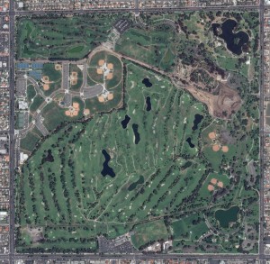 A 50-cm color image of Mile Square Golf Course in Fountain Valley, California collected on April 12, 2013 by Pléiades 1A. To see this course in 1.5-meter resolution, check out this month’s feature on SPOTMaps. Image photo enhanced by Apollo Mapping. © CNES 2012, Distribution Astrium Services / Spot Image S.A., France, all rights reserved.
The courses are settled within Mile Square Regional Park, which is operated and maintained by the County of Orange. Mile Square Golf Course is however owned and operated privately by a small group of partners. Both courses are open every day, each sending roughly 80-90,000 golfers through 18 holes a year.
The courses are comprised of mainly Kikuya Grass roughs and fairways, while the greens are Poa Annua and bentgrass. Due to a very mild climate, a lack of rain and highly saline irrigation water, the turf stands must be routinely cultivated with care in order to provide for optimal growing conditions. Mile Square sits on some of the lowest ground in the entire Los Angeles basin. Fountain Valley was named after several natural springs in the area, as well as its shallow water table.
As a side note of interest, Mile Square Golf Course is the number one course of actor Will Ferrell. So the next time you are in the Los Angeles, take a few hours out of your trip and play a round (or two) at Mile Square!
A special thanks goes out to Justin Harmon, our staff writer, and David Ahlstrand, superintendent of Mile Square, for their help writing this article.
The Pléiades 1 High-Resolution Satellite Constellation
The Pléiades 1 constellation (or at least part of it!) has been in orbit since December 2011 and if you have not had a chance to check out any sample imagery, take a few moments and have a look at the gallery on our website. If you work with high resolution imagery, you should consider Pléiades 1 for your next geospatial project.
A variety of Pléiades 1 products are available from both a growing archive and as a new collection, including 50-centimeter (cm) pansharpened imagery and 50-cm panchromatic–2-meter (m) 4-band multispectral bundles. We are happy to discuss the technical specifications, pricing and tasking options available with this new satellite constellation as Pléiades 1A has been joined in space by its twin, Pléiades 1B, which is now fully operational.
Working with Pléiades 1 for the past year plus, we have noticed that:
- Astrium is able to deliver on their tasking feasibilities.
- The data is crisp with excellent color saturation so that it is on par with competitors’ 50-cm satellites.
The Apollo Mapping sales team can answer any questions you might have about the high resolution satellite constellation, Pléiades 1. We can be reached anytime at (303) 993-3863 or sales@apollomapping.com.
More sample images and technical information about Pléiades 1A and 1B can be found on our website here.
