

An ethnographic map of the Philippines in the 1890s.
 Provincial negrito presence circa 1903 according to the maps from the Census of that period.
The Philippine “negrito groups” comprise a diverse amalgamation of people speaking over 30 different languages who are spread across the archipelago, mostly in the areas near the Luzon Island in the north and the Visayas and Mindanao in the south. The negritos have very dark skin and are often attributed the “pygmy” moniker due to their size and stature. A favorite group of people studied by anthropological ethnographers, past scholarly works have painted what has become known as the “negrito myth:” small in size, kinky hair, wearing a thong, living in bands and roaming the forest for food. Even the term ‘negrito’ is scoffed at as being culturally insensitive. This study looked at in this article uses the term not in defiance of respect to the group, but because there lacks an appropriate name to give them otherwise.
The study examined here set out to use GIS to map the displacement of negrito groups throughout the Philippines using historic data and more recent figures from the 2000 Philippines census. Negrito populations have been on the decline since the early 1900s, so the study’s purpose was to map migration and settlement patterns; as well as look for clues why some areas hosted stable numbers.
The negrito people have been studied, or at least marveled at, for centuries. A Spanish explorer who accompanied Magellan made note of them in the early 1500s, and further Spanish expeditions in the area led crusaders to be mystified by their existence. European scholars in the late 1800s studied the people and their culture, many of the anthropologists believing they had found one of the more primitive and indigenous people on our planet.
Contemporary negrito research has come to show that the early academic studies, while by some accounts were reductive, actually were very accurate in terms of their renditions of habits, interactions and livelihoods. This study’s author spent significant time on the ground, documenting observations and surveying the lands while referencing historic maps. These historic maps helped the author understand dispersal patterns and were combined with remote sensing and GIS analysis to fill in the gaps of past research and correct inconsistencies.
This study showed that the distribution of negritos has changed very little in the years since the earliest maps were made. It was found that the negritos occupy seven regions, consistent with the maps made a century ago. However, there was some migration to highlight caused by the encroachment of settlers, hunting ranges and forest tracts expanded by the government. This actually led to contention between the negritos (and other indigenous groups) and the new settlers over available resources. Due to state interference, negritos have in some cases abandoned their traditional lands to move deeper into the forest. In addition, a number have been moved to state reservations. As one can imagine, the negritos yearn for their old autonomous lands; hopefully this study, and others like it, will bring relief to their plight.
Justin Harmon
Staff Writer
Have you checked out the new and improved Image Hunter yet?!?! If not, you should!
Listening to the feedback we received on improving imagery search engines, the new version of Image Hunter features a major overhaul to the user interface as well as to the backend architecture. Image Hunter Version 2 is built on open-source technology so now it works on all computers, not just on Windows machines. We slimmed down the user interface to make it easier to find the imagery filters and other available tools. All things said, we really think you will enjoy your browsing experience with Image Hunter (Version 2).
Key May 2014 Improvements
This month, we upgraded the backend spatial databases to make imagery searches and shapefile/KMZ uploads more stable.
Image Hunter can be accessed 24 hours a day, 7 days a week and is a one-stop shop for every major source of medium and high-resolution satellite imagery on the market today, including:

- WorldView-2
- QuickBird
- WorldView-1
- GeoEye-1
- IKONOS
- The Pléiades 1 constellation
- The entire SPOT constellation
- RapidEye
If any of our readers have struggled with other geospatial search engines that are clunky, only query one data source and/or do not provide image previews, then Image Hunter is the solution to your woes, as it features:
- Online browsing of satellite imagery from 3 data providers and 14 satellites.
- Near-instantaneous loading of low resolution preview imagery with collection date, cloud cover and other key metadata.
- The ability to define your area of interest by address and with coordinates, geometric shape or shapefile/KMZ.
- A responsive basemap with street names to provide spatial context when discovering data as well as crowd-sourced updates for the most accurate map possible.
- Exports of the area of interest you create as well as the scenes you select in shapefile or KMZ format.
- Support for all operating systems, and not just our friends with Windows machines!
The new version of Image Hunter can be accessed here. We are excited to find out what you think about Version 2!
If you have any ideas and/or feedback to improve the new Image Hunter, please let us know at sales@apollomapping.com or (303) 993-3863.
Sometimes one Geospatial Frequently Asked Question (G-FAQ) leads me directly into my next topic, and that is the case this month. While doing research for the four part series on ‘What is GIS?’, I realized that I had a gap in my GIS knowledge on topology. There is not a day that goes by where I am not learning something new and this G-FAQ is no different. So without further ado, let’s jump into an exploration of spatial topology in the world of GIS.
This two-part G-FAQ on spatial topology will focus on three core questions:
What is spatial topology, why is it important and how is it maintained in GIS? What are example files types that are topological in Esri’s ArcGIS? Do shapefiles have topology?
Before we jump head long into this discussion on spatial topology, let me start with a high-level definition. Topology is the science and mathematics of spatial relationships of vectors in GIS. There are four basic spatial relationships that can be maintained with vector features, I will elaborate on these shortly: adjacency, connectivity, containment and coincidence. These spatial relationships are recorded in topological vector models with the assumption of a two-dimensional world (i.e. all of the features are on the same plane). Keep in mind that raster files do not have topology–for a detailed handling of vector versus raster file types, please refer to the April 2014 G-FAQ edition.
As a quick side note, similar to the last few G-FAQ’s, this edition will also focus on Esri’s ArcGIS with regards to topology–though I do assume (perhaps incorrectly!) that these relationships are maintained likewise in all GIS software.
Arc-Node Data Structure
 No single image can illustrate all of the possible arc-node relationships and then the lists that are created for each type of vector–but what you see here is the closest I could find. Also keep in mind that there are different theoretical constructs for describing arc-node data structures, I choose the version that made the most sense. At the top of the graphic are points and then the subsequent list made for these vectors. Below this are lines and their related lists–I have added a direction arrow to the original graphic to illustrate arc directionality. Also keep in mind that where there are “…” in the Left Poly column, this equates to the universe polygon mentioned here. At the bottom is a polygon and then one of the two lists mentioned here (i.e. the polygon-arc list). (Image Credit: Hunter College)
Spatial topology in ArcGIS is predicated on the vector arc-node data structure. As was mentioned in the April 2014 G-FAQ, there are three basic types of vectors, i.e. points, lines (or arcs) and polygons. Here are the basic rules of the arc-node data structure:
- All arcs are comprised of nodes with 0 to more vertices in between.
- A node is at the start and end of each arc. As there is a start and end to arcs, they have a direction in which they are created.
- Vertices between nodes define the shape of arcs. You can think of vertices as points along the curve of an arc.
- Arcs can be connected and if they are, they share a common node.
- Connecting arcs in a close geometric shape creates polygons.
- When arcs are connected to make a polygon, it actually defines two polygons. The first is often called the ‘universe polygon,’ which is all of the space outside the defined shape. The second is the area contained within the connected arcs.
Each of the arc-node relationships defined above are stored in lists. For points, the list contains an identifying number and its X and Y position (or coordinate).
For lines, the list contains an arc number, the start and end node numbers and thus the direction of the arc (i.e. clockwise or counter-clockwise) is inferred here. There is also an arc-coordinate list that contains the arc number and the associated X and Y coordinates.
For a polygon, there are also two lists. The first is the polygon-arc list which contains an identifying polygon number and then the arc numbers that comprise it. The second is the left-right list which contains the arc number and then the identifying number of the polygons to the left and right of the arc.
The Types of Spatial Topology and the Files That Maintain It
As has been discussed in previous G-FAQ editions, there are four basic types of spatial topology that can be maintained:
- Adjacency–which vector features are next to each other?
- Connectivity–which arcs connect to each other?
- Containment–which vector features are within other polygons?
- Coincidence–which vector features occupy the same space?
 Admittedly the four types of spatial topology listed here have been extremely simplified and lumped together for the benefit of our readers. If you want to see all of the spatial relationships possible in ArcGIS, get ready for your mind to spin a bit. Here is an extensive look at all of the topological rules you can implement in geodatabases between points, lines and polygon vectors. (Image Credit: Esri)
In ArcGIS, there are two key file types that maintain topology, ArcINFO coverage files and geodatabases. The reason I say key file types here is to allow some wiggle room as admittedly there may be other file types with topology but I was unable to uncover any in my research. If our readers know of additional file types with explicit spatial topology, please leave a comment below so the rest of us can learn even more!
ArcINFO coverage files are rarely used today, well at least in the GIS work that I have done. They can be thought of as the original Esri shapefiles. By definition, a coverage file is topological as a topology table is created and maintained as the file is modified and expanded upon. Coverages are a collection of various files, the topology table is one of them, and they have a complex structure as you see in the case of a geodatabase. A coverage can contain point, line and polygon features in a single file. Often times, you will see coverages grouped into a single file with the extension .e00–these are called ArcINFO Export files and need to be extracted first before they can be read by ArcGIS. One tool you can use to extract ArcINFO Export files is offered for free from Esri here, it is called Import71.
Geodatabases are by far the more popular file format that can maintain topological relationships; and I say they can maintain topology as it is possible to create a geodatabase without these rules embedded. A geodatabase can also contain point, line and polygon layers which are called features. In order to embed topology in a geodatabase, it is necessary to define classes of features and the rules that relate them to each other. Topology can be maintained between points, line and polygons. Once these rules are validated, the set of features will be related through topological relationships that are maintained even when you edit. It is possible to create exceptions to these topological rules so they can be violated in specific instances but then maintained across the broad set of related features.
There are two key differences with regards to spatial topology of ArcINFO coverage files and geodatabases. First, in coverage files, there is a specific table defining all the topological relationships between the features that is created and changed as the file is edited. And for a geodatabase, there is not a specific table but rather a set of rules that are stored to maintain topology. Second, with a geodatabase it is possible to edit a set of feature classes that share a common geometry, while in coverage files each vector layer must be edited independently. So for example take two polygon layers representing parcels and easements in a city where they share a common geometry (or boundaries). When the parcel layer is edited in a geodatabase, so is the easement layer; while in a coverage file, it would be necessary to edit both layers independently.
By now, I am sure our readers’ heads are full of fun information on arc-node data structures and spatial topology, so for now, let’s call a close to this two-part G-FAQ. In the next edition, we will pick up this discussion, looking at why spatial topology is (or perhaps was…) important and at the ‘topology’ of shapefiles.
Do you have an idea for a future G-FAQ? If so, let me know by email at brock@apollomapping.com.
Find Out More About This Topic Here
- Esri–ArcGIS: Working with Geodatabase Topology
- Oberlin College–Understanding Topology
- Saint Louis University–How to Create and Edit Topology
- State University of New York–Data Structures
- University of Eastern Michigan–Fundamentals of GIS Data
- University of Massachusetts–Topology Slides
- University of Nebraska, Omaha–Structuring Maps
- University of North Texas–GeoDatabase Topology
- University of Texas–Vector Data Model
- University of Washington–Spatial Data Model
Brock Adam McCarty
Map Wizard
(720) 470-7988
brock@apollomapping.com
- For this month’s focus on technology, let’s take a look at several recent advancements in the biofuel industry.Bacteria are often the powerhouse that convert raw biomatter to ‘fuel.’ This research has bioengineered E. coli to convert biomatter to long-chain fatty acids which are the precursors of gasoline. These researchers have inserted tree enzymes into bacteria in order to produce pinene, a high-octane hydrocarbon that could replace rocket fuel. And this research inserts a bacterial gene into E. coli to increase the efficiency of biofuel production by strengthening the cells.
Increasing the sources of biomatter will obviously make biofuels more sustainable as the use of them grows; and so here are two ideas for new sources: coffee grounds and alligator fat. Finally, improving the efficiency of biofuel production can also include pathways other than conversion by microorganisms. For instance, this research which uses solar energy to create synthetic fuels; this idea uses an acid wash to produce acetone from corn husks; or this technology to convert ethanol to transportation-ready fuels.
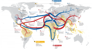 Map showing the spread of leprosy, malaria and small pox across the globe as well as an indication of the time of infection.
- Maps often paint pictures we cannot with words alone. And here is a map that is no exception to the rule. It shows the spread of malaria, leprosy and small pox across the world from their points of origin. While leprosy and small pox have been eradicated, malaria still kills at least 1 million people per year.
- I am not what you would call an outdoorsy person, but I do respect nature! And in honor of warm weather activities, this month I Googled, “fishing and GIS.” Here is an interesting PowerPoint put together by Wedell (Oregon State University) and Revell (U California Santa Cruz) that shows the power of GIS for community-based fisheries management. In this study, the authors employ participatory GIS to gauge local knowledge of fishing habitats, use of these areas and (of course) to create maps.
- From the Gulf of Mexico, we travel to the northeastern edge of our country with an exploration of Portland, Maine’s GIS resources. The City of Portland GIS offers both a web application and PDF versions of the maps they produce. There are more than 60 PDFs that can be viewed and downloaded from this page, however the vast majority of the links seem to be broken. The GIS department also created 12 online maps of various themes including a parcel viewer that lets users search for a parcel and then query detailed assessor information. The online maps also let you print your current screen view. Finally, you can download the ArcGIS mobile app, search for Portland Maine and then view parcel and planning data on your smartphone.
Brock Adam McCarty
Map Wizard
(720) 470-7988
brock@apollomapping.com
In this monthly article, we provide details on updates to Airbus Defense and Space GEO’s SPOTMaps product. SPOTMaps is an orthorectified 2.5-meter (m) and now 1.5-m natural color imagery layer with coverage over more than 100 countries–totaling an impressive 108 million plus square kilometers (sq km). For projects requiring a value-priced basemap better than what 15-m Landsat can offer, there is no other choice than SPOTMaps.

 1.5-meter SPOT 6 natural color images collected over Congressional Country Club and Bethesda, Maryland on August 15, 2013. If you would like to see this golf course in Pléiades 1 50-cm resolution as a comparison, please click here. © CNES 2012, Distribution Airbus Defense and Space / Spot Image S.A., France, all rights reserved
 This map of SPOTMap1.5 coverage shows the regions that have been released as well as those currently in production. An Apollo Mapping representative can provide more details on the specific year ranges used in each mosaic.
 This map of SPOTMap2.5 coverage has been color coded to show the collection year which makes up the majority of each mosaic as well as those markets that were added in the final month of production (i.e. August 2013). An Apollo Mapping representative can provide more details on the specific year ranges used in each mosaic.
SPOTMaps Product Updates–May 2014
- 22 million sq km of SPOTMap1.5 coverage is to be released in 2014 alone!
- These countries are currently in production and will be added to the SPOTMaps1.5 database soon:
- Iran (part of the country)
- Iraq (part of the country)
- New Zealand
- Niger
- Oman
- Saudi Arabia (part of the country)
- South Africa (most of the country)
- United Arab Emirates
- Yemen
- Production of SPOTMaps2.5 is complete now that SPOTMaps1.5 are being released.
For those who have never worked with SPOTMaps, below is a summary of key product specifications of the 1.5-m and 2.5-m versions as well as product differentiators.
Key Product Specifications
- SPOTMaps1.5
- Resolution: 1.5-m
- Spectral Bands: true natural color (RGB)
- Horizontal Accuracy: 6 to 10-m CE90 (circular error 90%)
- Projection/Datum: UTM WGS84
- Source Data: SPOT6/7 satellite imagery
- File Format: GeoTIFF
- SPOTMaps2.5
- Resolution: 2.5-m
- Spectral Bands: simulated natural color (RGB)
- Horizontal Accuracy: 10 to 15-m RMSE (root mean square error)
- Projection/Datum: UTM WGS84
- Source Data: SPOT5 satellite imagery
- File Format: GeoTIFF
Product Differentiators
- Recent and ready for immediate delivery and integration with your GIS
- Seamless, orthorectified coverage across countries and entire regions in 1.5-m and 2.5-m resolution
- Suitable for work up to 1:10,000 scale
- Custom product framing with minimum orders of ~100 sq km
- Product series is updated nearly every month
- Source data can be delivered with all SPOTMaps mosaics
- Volume and academic discounts are offered
- Multi-user licenses are available
If you would like pricing details and/or additional product details, such as date ranges and accuracy specifications, please let us know at sales@apollomapping.com or (303) 993-3863.
In this monthly feature, we span the globe to examine Our Changing Landscape with time series of medium resolution RapidEye satellite imagery. The RapidEye archive dates back to late 2008 and already contains more than 5 billion square kilometers of data. This month, we look at the harvest of tulips in Den Burg, Netherlands.
The RapidEye Constellation
RapidEye is a constellation of five 5-meter medium resolution satellites each offering five spectral bands of information. The RapidEye constellation offers daily revisits to every location on the planet with a huge footprint that is 77-km wide. The data is priced competitively with a starting cost of $1.28 per square kilometer for all five spectral bands–academics do receive discounts. RapidEye adds a fifth band, the red edge, to the ‘traditional’ multispectral set of blue, green, red and near-infrared (NIR). The additional spectral data in the red edge band allows users to extract more useful land ‘information’ than can be from traditional 4-band imagery sources. When RapidEye imagery is ordered as a Level 3A Orthorectified product, images from multiple dates are extremely well registered, making it the ideal data source for Our Changing Landscape.
Netherlands Tulip Harvest–Den Burg
 Click on the image above to see an animation of 5-meter natural color imagery collected over Den Burg, Netherlands on March 23, 2011, May 1, 2011 and October 15, 2011. In this animated series, you can see significant changes in the ground cover of many of these fields. (Images Courtesy: RapidEye)
A tulip is a flowering perennial plant (meaning it lives for two or more years) that grows from bulbs. The term is used to broadly describe about 100 plant species belonging to the Liliaceae family, however few are found outside of gardens and greenhouses. Tulips are native to the Mediterranean climate found in Europe, northern Africa and the Middle East, with some species extending through the mountains of Iran to northwest China. Tulip flowers have three petals and three sepals and come in a wide variety of colors.
Tulips grow the best in well drained soils and in areas with long, cool springs and then dry summers. In order to be grown from a bulb, tulips require a period of cool weather, called vernalization, as such they are often planted in late-summer to early-fall. Bulbs are planted from 2 to 8 inches deep in soil; the deeper they are, the longer the stem is when they are harvested. When grown from a bulb or a tissue culture, tulips will maintain their genetic integrity (i.e. they will look the same as their parents); and when grown from seeds, new hybrid species are created which look different from their parents.
The Netherlands is the world leader in tulip production, growing an estimated 4.3 billion bulbs each year, of which 2.3 billion are made into cut flowers. Approximately 40% of these cut flowers are exported outside Holland, with the majority staying in Europe. The Netherlands is an ideal climate for growing tulips with its long, cool springs and moist, well-drained soils. The peak season for tulip blossoms is from mid-March to the end of May. Tulip farms in the Netherlands cover about 11,000 hectares and are mechanically harvested given the sheer volume of fields that are planted. The Netherlands accounts for nearly 90% of the world’s total area of tulip farms planted each year!
If you would like to find out more about using RapidEye for your academic studies, engineering projects or any landscape analysis, let us know at sales@apollomapping.com or (303) 993-3863.
It has been a while since I featured a collection of free vector and raster files, so let’s reverse that trend this month. The folks at Natural Earth Data have a very nice collection of free GIS data that is both easy to download and also offered in various scales. This collection of free data is pretty self explanatory so let me give our readers a sense of what you can download in either small, medium or large scale:
 A sample of the large-scale Natural Earth 1 with Shaded Relief dataset (no water is included in this version) over the Midwest of the United States.
- Cultural Layers
- Country boundaries and administrative units
- Disputed areas
- Populated places
- Railroads
- Airports
- Ports
- Urban areas
- Parks and protected lands
- Timezones
- Physical
- Coastline
- Land masses
- Minor islands
- Reefs
- Ocean
- Rivers and lakes
- Major physical features
- Playas
- Ice shelves and glaciers
- Bathymetry
- Worldwide color and grey-scale raster backgrounds
Until my next edition of Free For All, happy hunting for free geospatial goodies!
Brock Adam McCarty
Map Wizard
(720) 470-7988
brock@apollomapping.com
We are pleased to announce that sales of the much anticipated WorldDEM produced by Airbus Defense and Space are under way! For the past three years, Airbus’ twin high-resolution radar satellites, TerraSar-X and TanDEM-X, have imaged the entire land surface of our planet multiple times to create the first ever global 12-meter (m) elevation model. The WorldDEM is ideal for all mapping projects requiring accurate elevation models including orthorectification, floodplain determination, mineral exploration and hydrocarbon development.
 A comparison of 30-m SRTM and 12-m WorldDEMTM elevation data over Arkansas, USA.
WorldDEM Specifications
The key product specifications of Airbus’ WorldDEM are as follows:
- Resolution: 12-m
- Coverage: entire landmass of the Earth, ~150 million square kilometers (sq km)
- Absolute Vertical Accuracy: 4-m Linear Error 90% (LE90)
- Relative Vertical Accuracy: < 2-m LE90 (slopes ≤ 20%), < 4-m LE90 (slopes > 20%)
- Absolute Horizontal Accuracy: < 10-m Circular Error 90% (CE90)
- Vintage: all data collected within 3 years
- Source: interferometry from synthetic aperture radar (SAR) satellites TerraSAR-X & TanDEM-X
- Minimum Order: 500 sq km per polygon
- File Format: GeoTIFF
- Projection: geographic WGS84 (EGM2008, vertical datum), meter vertical unit
- Product Line Options:
- WorldDEMcore–unedited digital surface model (DSM), includes spikes, wells and voids
- WorldDEMTM–a DSM with removal of artifacts and water body flattening
- WorldDEM DTM–artifacts and surface features removed, i.e. a digital terrain model (DTM)
WorldDEM Coverage and Pricing
WorldDEM data has a 500 sq km minimum order size with a 10-km width requirement. Prices for two of the product lines have been set:
- WorldDEMcore–$10.80 per sq km
- WorldDEMTM–$13.50 per sq km
Currently, there are portions of the United States, Canada and Australia that are ready for production. In the coming months, the rest of the world will be released. For the estimated release dates of regions not currently ready for production, please email the Apollo Mapping team at sales@apollomapping.com.
 A coverage map of the one-degree cells that are currently ready for production. All of the regions on this map are either red (i.e. pre-production phase) or yellow (ready for production). Areas that are ready for production will take approximately four (WorldDEMcore) to eight weeks (WorldDEMTM) to deliver once an order is placed.
WorldDEM Samples
You can download three 12-m WorldDEMTM samples here:
- Buraydah, Saudi Arabia–desert with agriculture present; 576 m to 737 m
- Mjosa Lake, Norway–hilly terrain with large water bodies; 100 m to 840 m
- Wagga Wagga, Australia– forest and urban with many water bodies; 137 m to 922 m
For more information about 12-m WorldDEM data, please send us an email at sales@apollomapping.com.