
For projects requiring a more detailed look than can be offered by the common free sources of elevation data and for those in cloudy or hard-to-reach regions where this data is of poor quality, Astrium GEO’s Elevation10 product suite is the ideal solution. Elevation10 is a 10-meter digital elevation model (DEM) derived from stereo pairs collected by the radar satellite, TerraSAR-X. These DEMs are often delivered within a month of order placement utilizing data obtained in the past two years.
TerraSAR-X is a synthetic aperture radar (SAR) satellite, meaning it is an active sensor unlike the optical satellites most of us are familiar with such as QuickBird, Pleiades 1 and WorldView-2. An active sensor (1) creates an energy pulse, in this case radar waves; (2) aims them at a surface, in this case our planet; and then (3) very accurately measures the amount of time it takes for this pulse to return to the sensor. Radar waves can pass right through clouds which are an optical satellite’s worst nightmare.
As TerraSAR-X measures the time it takes for energy pulses to return to its sensors as well as its position in space in the XYZ directions, radar stereo pairs have higher accuracy than do traditional pairs collected by optical satellites. This means that elevation data extracted from TerraSAR-X stereo pairs is accurate even without the use of ground control points. Ground control points can be expensive to collect–particularly in remote and unsafe areas–so this can be a significant cost savings vis-à-vis other elevation products.
 Click on the image above to see an animated comparison of 10-meter Elevation10 (both a DSM and DTM), 30-meter ASTER GDEM and 90-meter USGS SRTM data over Barcelona, Spain. (Image Sources: USGS, JPL and Astrium GEO)
Elevation10 is created from TerraSAR-X radar stereo pairs collected in StripMap mode. StripMap data has resolution up to 3-meters with a footprint that is 30 kilometers (km) wide by 50 km long. By employing TerraSAR-X stereo pairs collected in both ascending and descending directions, Astrium GEO is able to remove many of the anomalies that are common in SAR elevation data.
Elevation10 is offered as both a digital surface model (DSM) which includes vegetation, buildings and other human-made structures; and as a digital terrain model (DTM) where these have been removed. DTMs are hydrographically enforced to make sure that features which impact water flow, such as dams and embankments, are represented. Hydrographic enforcement is also offered with DSMs. The accuracy specifications for Elevation10 are as follows:
- Absolute Horizontal Accuracy–5 to 10 meters (Circular Error 90%, CE90)
- Absolute Vertical Accuracy–5 to 10 meters (Linear Error 90%, LE90)
For regions of the world with limited access, such as the Himalayas and the Andes, or in regions with persistent cloud cover and/or haze, such as Malaysia and Beijing, Elevation10 is the ideal solution. Elevation10 data is priced by the square kilometer according to the product type with academic discounts available. For more information about Elevation10, contact your Apollo Mapping sales representative at (303) 993-3863 or sales@apollomapping.com.
In this monthly piece, we give our readers a sense of the high-resolution imagery coverage collected over a geography during a specified window. To do this, we pick a high resolution satellite, a defined time period and area of interest, then report key statistics on the total amount of imagery collected in square kilometers (sq km). Without further delay, let’s jump into our analysis.
 This map shows the areas imaged by the WorldView-2 constellation from June 1 to August 31, 2014 over the continental USA. Please note that in many instances, multiple images were collected over the same area which is difficult to portray on this static map.
Graphic Region of Interest: continental USA
Land Mass Covered: 7,779,029.0 sq km
Time Period: June 1 to August 31, 2014
High Resolution Satellite: WorldView-2
WorldView-2 Constellation Imaging Statistics–Continental USA
Total Area Collected: 4,523,772.3 sq km; 49,171.4 sq km per day
Area Collected @ 20% or Less Clouds & 30 Degrees Off-Nadir: 2,513,386.5 sq km; 27,319.4 sq km per day; 55.56% of total
Continuing with the theme of ArcGIS lessons started in December’s Geospatial Frequently Asked Question (G-FAQ), this month we look at the steps required to calculate the area of a polygon shapefile. In this G-FAQ, we cover some of theory behind calculating areas in ArcGIS and then also offer a short video showing you the exact steps required to complete the calculation.
Specifically, this G-FAQ will address the following set of core questions:
What is the easiest way to calculate the area of a polygon file in ArcGIS 10.x? What projection does the data need to be in to support this calculation? What field type should I use for area calculations?
Before you watch the short video accompanying this G-FAQ, take a few moments to read through some of the theory behind area calculations in ArcGIS. We have ordered the information below to mimic the steps taken in the video.
Choosing the Correct Projection
In order to complete an area calculation for a polygon shapefile, it needs to be in a projected coordinate system as opposed to geographic, as a geographic system projects data on to a round surface so it is impossible to accurately measure distances, areas, etc. Data in a projected coordinate system is displayed as if sitting on a flat plane so it is now possible to accurately calculate distances, areas, etc.
If you are working with polygons in a small area, you can chose a local projected coordinate system that you commonly work in, for instance UTM. However, for area calculations that include polygons spread over a large region, you will need to choose an equal-area, global projected coordinate system. A projected coordinate system can prevent distortion in one spatial dimension but will then always distort in another. Projected systems can control for: equal area, equal distances, equal angles, direction and scale; but they cannot control for all at once.
My equal-area, global projection of choice is: Cylindrical Equal Area (World). It models the world with perpendicular latitude and longitude lines. Longitudes are spaced equally while latitudes are unequally spaced to account for the shrinking volume of our global as you move to the poles. A WGS84 datum is used as it is the mostly widely accepted global datum. There are other equal area projections you could choose, for instance you can shift the latitude lines used for baseline calculations farther north to de-emphasize area miscalculations in high latitudes.
Choosing the Correct Field Type
Once you have re-projected your data into the equal-area system of your choice, it is time to add a field to your attribute table to hold the area calculations. We will walk you through the exact steps of doing this in the short video that accompanies this G-FAQ, but for now a bit of theory behind the field types you can add. For numeric values, you are able to create these types of fields (or columns):
- Short Integer–numbers without decimal places between -32,768 and 32,767
- Long Integer – numbers without decimal places but of any length or number of digits
- Float–numbers with decimals with less than 7 digits total (including decimal places)
- Double – numbers with decimals and no length limit
For each of these four field types, you are also able to define the precision and scale for the new column. Precision equals the total number of digits you can store and is an option for all four field types. Scale is the total number of decimal places and so is only an option for float and double field types.
When I calculate polygon areas in Arc, I typically choose a double field with “20” for precision and “10” for scale.
Comparison of Area Calculations With Different Equal-Area Projections
We have one final item to cover quickly before you check out the short video here. To show you how close equal area projections are to each other, I projected the same shapefile into three different systems. The polygon file I used spanned the globe and contained 176,987 individual polygons. Here is the total area calculated by each of the three equal-area projections:
- South Pole Lambert Azimuthal Equal Area–256,117,937.745012 square kilometers (sq km)
- Sphere Cylindrical Equal Area–255,623,570.713166 sq km
- World Cylindrical Equal Area – 256,123,154.208427 sq km
To put these figures a different way, if you set the total area calculated by World Cylindrical Equal Area as the ‘true value’ then here is how close the other two projections come:
- South Pole Lambert Azimuthal Equal Area–99.998% of the true value
- Sphere Cylindrical Equal Area–99.805% of the true value
So then, what you see from these comparisons is that shifting the baseline latitude line north or south has little impact on the final area calculations as the South Pole equal area projection was very close to our true value. The bigger impact on these calculations is the datum used in the re-projection as Sphere Cylindrical Equal Area is much farther off since it uses a spherical representation of the globe; and not the most widely-regarded (and accurate) global datum, WGS84, used in the other two projections.
Do you have an idea for a future G-FAQ? If so, let me know by email at brock@apollomapping.com.
Find Out More About This Topic Here
- State University of New York, Syracuse–About XY Domain & Precision in ArcGIS
- University of California, Santa Barbara–Lecture 5
- University of Colorado–Map Projection Overview
- University of Maine–Coordinate Systems and Map Projections for GIS
- University of Notre Dame–Creating Vector Data in ArcGIS
- University of Washington–Projections and Coordinate Systems
Brock Adam McCarty
Map Wizard
(720) 470-7988
brock@apollomapping.com
From our home state of Colorado, we head west for this stop on the Pléiades 1 Golf Course of the Month at the Arnold Palmer Course of PGA WEST in La Quinta, California, the site of the Humana Challenge in partnership with the Clinton Foundation from January 22nd to the 25th. The event has been played since 1960 and was originally known as the Palm Springs Desert Classic but more famously as the Bob Hope Classic. The Humana Challenge is an official US PGA Tour event with a $5.7 million purse and a pay-out of $1.026 million and 500 FedExCup points to the winner. But this tour event is definitely best known for its mixed celebrity and professional charity competition that has drawn the likes of Bill Clinton, Bing Crosby, Dwight Eisenhower and Kirk Douglas. In the charity competition, 156 celebrity amateurs play alongside the 156 professionals in rotating pairs for the first two rounds of the tournament. Since 1960, the Humana Challenge has raised more than $52.5 million for local nonprofits, including the Eisenhower Medical Center.
 A 50-cm color image of PGA WEST’s Arnold Palmer Course collected on September 21, 2014 by Pléiades 1A. To see this course in 1.5-meter resolution, check out this month’s feature on SPOTMaps. Image photo enhanced by Apollo Mapping. © CNES 2012, Distribution Airbus Defense and Space / Spot Image S.A., France, all rights reserved.
PGA WEST is a large golf club consisting of six world renowned courses including Arnold Palmer (site of the Humana Challenge) and TPC Stadium. Designed by Pete Dye and opened for play in early 1986, in its brief 29 year history, the six courses have won a plethora of domestic and international golf awards. Located in sight of the Santa Rosa Mountains, the Arnold Palmer course has a traditional play with rolling Bermuda grass fairways and multiple water hazards. The course plays 6,930 yards from tournament tees at a 72 par. The longest hole is the relatively flat par 5 6th at 562 yards; and the shortest is the downhill par 3 17th at 130 yards.
The golf legend Arnold Palmer is the tournament’s most decorated winner, capturing the event 5 times in 1960, 1962, 1968, 1971 and 1973. Last year’s winner was American golfer Patrick Reed with a two-stroke lead over runner up, Ryan Palmer. While the field was not set for the event at the time this article was written, the Humana Challenge is sure to be an early season PGA Tour pleaser!
The Pléiades 1 High-Resolution Satellite Constellation
The Pléiades 1 constellation (or at least part of it!) has been in orbit since December 2011 and if you have not had a chance to check out any sample imagery, take a few moments and have a look at the gallery on our website. If you work with high resolution imagery, you should consider Pléiades 1 for your next geospatial project.
A variety of Pléiades 1 products are available from both a growing archive and as a new collection, including 50-centimeter (cm) pansharpened imagery and 50-cm panchromatic–2-meter (m) 4-band multispectral bundles. We are happy to discuss the technical specifications, pricing and tasking options available with this satellite constellation.
Working with Pléiades 1 since the launch of the first twin satellite, P1A, we have noticed that:
- Airbus Defense and Space is able to deliver on their tasking feasibilities.
The Apollo Mapping sales team can answer any questions you might have about the high resolution satellite constellation, Pléiades 1. We can be reached anytime at (303) 993-3863 or sales@apollomapping.com.
More sample images and technical information about Pléiades 1A and 1B can be found on our website here.
In the coming months, Apollo Mapping will be unveiling the industry’s most affordable, scalable and secure spatial cloud, the GISrack. While we are busy building out the infrastructure and technology required to support the most flexible GIS cloud on the market, now is a great time to explain a bit about the GISrack.
Some of you may have used other GIS cloud services in the past, and in many ways the GISrack will be similar to these. But the GISrack will distinguish itself in a variety of important manners. Here is a list of the key features that will be unique to the GISrack:

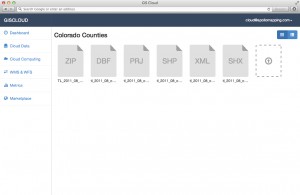

- Near-instant set-up–unlike other GIS clouds, the GISrack will take less than five minutes to sign up for, load data on to and get started using. No other cloud comes close to that flexibility.
- Tons of free spatial data–included with every subscription is access to more than 4 terabytes (TB) of free vector and raster data covering the United States and many parts of the world.
- A marketplace for spatial data – all users will have access to a library of spatial data that can be added to your GIS cloud. Further, users will be able to post data they have created to the marketplace to sell to other users (or let them use for free if you wish).
- Cloud computing – we will ask all users for feedback on the spatial operations they perform most frequently and will then implement the most popular ones in the GISrack.
- Free entry-level subscriptions – users will be able to use the full-functionality of the GISrack with up to 25 megabytes (MB) of free storage and bandwidth. And once you pass this storage limit, subscriptions will start at just $5.00 per month!
- A robust online viewer–for those users in your organization lacking access to a GIS application, the GISrack will feature an online viewer that can be accessed from anywhere in the world as long as users have internet access.
- Enhanced browsing speeds – we will have all of your spatial data cached in multiple locations around the world so access times will be greatly reduced for international users.
- Flexible streaming architecture – administrators will be able to setup multiple WMS and WFS feeds that can be shared with the appropriate teams of data users. Each feed can be seeded with the datasets these users need access to.
- Industry-leading data redundancy – with 99.999999999% data redundancy, you can be assured that your data will not be lost once placed on the GISrack.
Do you have any specific questions you would like answered about the GISrack? Or perhaps you want to join the beta program? If so, let us know by email at sales@apollomapping.com.
In this monthly feature, we span the globe to examine Our Changing Landscape with time series of medium resolution RapidEye satellite imagery. The RapidEye archive dates back to late 2008 and already contains more than 5 billion square kilometers of data. This month, we look at changes in one of the largest open pit mines in the world, Bingham Canyon Mine, Utah.
The RapidEye Constellation
RapidEye is a constellation of five 5-meter medium resolution satellites each offering five spectral bands of information. The RapidEye constellation offers daily revisits to every location on the planet with a huge footprint that is 77-km wide. The data is priced competitively with a starting cost of $1.28 per square kilometer for all five spectral bands–academics do receive discounts. RapidEye adds a fifth band, the red edge, to the ‘traditional’ multispectral set of blue, green, red and near-infrared (NIR). The additional spectral data in the red edge band allows users to extract more useful land ‘information’ than can be from traditional 4-band imagery sources. When RapidEye imagery is ordered as a Level 3A Orthorectified product, images from multiple dates are extremely well registered, making it the ideal data source for Our Changing Landscape.
Bingham Canyon Mine, Utah
 Click on the image above to see an animation of 5-meter natural color RapidEye imagery collected over the northern edge of Bingham Canyon Mine on July 1, 2010, August 14, 2012 and July 19, 2014. In this animated series, you can see significant changes along the mine walls and the supporting infrastructure in the two active zones at the graphics’ center. (Images Courtesy: RapidEye)
In 1848, two cattle ranchers, Sanford and Thomas Bingham, discovered copper ore on the ground of their family’s lands located some 25 miles from Salt Lake City, Utah. And this rather innocent discovery led to the opening of the world’s deepest mine in 1906 which is now 2.75 miles across and 0.75 miles down. Bingham Canyon Mine is also the world’s highest-yielding copper mine, producing more than 19 million tons in its 100+ year history. And the mine produces more than just copper as some 400,000 ounces of gold, 4 million ounces of silver, 30 million pounds of molybdenum and 1 million tons of sulfuric acid are extracted annually.
In the mid-2000’s, with a rise in copper prices, the current owners of the site, Rio Tinto, decided to open an underground mine which will produce enough ore to cover 24 blocks of midtown Manhattan. Rio Tinto also plans to expand the open pit mine by pushing back its south wall some 1,000 feet and digging down 300 feet to extract 700 million tons of additional copper ore. Mining on this scale is not without its hazards as an April 11, 2013 landslide attests to. In this disaster, some 165 million tons of rock tumbled over itself, causing a localized earthquake measuring 5.1 on the Richter scale which damaged infrastructure and mining equipment.
Before closing this Our Changing Landscape, here are some statistics that will help give you a sense of the scale of the massive mining operation at Bingham Canyon:
- Each day, some 450,000 tons of rock are taken out of the mine.
- 1,200 pounds of explosives are put into holes 55 feet deep to break up rocks and expose copper ore.
- This single mine produces about 17% of the US’ copper needs and 1% of the world’s each year.
- The April 2013 landslide was estimated to cut Rio Tinto’s yearly profits by 7%.
- The metals extracted from Bingham Canyon are valued at approximately $1.8 billion per year.
- If the open pit mine at Bingham were a stadium, it would hold more than 9 million people.
- Stacking two Willis Towers (formerly Chicago’s Sears Tower) end to end would still not reach the top of the mine.
- It would take more than 38 professional soccer pitches laid end-to-end to span the entire mine.
If you would like to find out more about using RapidEye for your academic studies, engineering projects or any landscape analysis, let us know at sales@apollomapping.com or (303) 993-3863.
 One of the first 1.5-m SPOT 7 images collected on July 3, 2014 of Paris, France. © CNES 2012, Distribution Airbus Defense and Space / Spot Image S.A., France, all rights reserved
Starting immediately, Apollo Mapping is pleased to announce that sales of Airbus Defense and Space’s medium resolution satellite, SPOT 7, have commenced. Launched on June 30th, SPOT 7 collects 1.5-meter panchromatic and 6-meter multispectral imagery over a swath that is 60-kilometers (km) wide. SPOT 7 and its identical medium-resolution satellite twin, SPOT 6, can image more than 6 million sq km of imagery per day or more than 2 billion sq km per year between them!
As a reminder to our readers, here is a summary of the key specifications of the medium-resolution satellites, SPOT 6 and SPOT 7:
- Resolution and Spectral Bands: 1.5-meter (m) panchromatic & 6-m multispectral (i.e. blue, green, red and near-infrared)
- Bit Depth: 12-bits
- Swath Width: 60-km (at nadir)
- Constellation Collection Capacity: 6 million sq km per day
- Minimum Order Size: 100 sq km (archive); 500 sq km (new collection)
- Commercial Starting Cost: $5.15 per sq km (archive); $6.20 per sq km (new collection); academic discounts are available
For more information about the SPOT 6–SPOT 7 constellation, please refer to our website here or send us an email at sales@apollomapping.com.
Have you checked out the new and improved Image Hunter yet?!?! If not, you should!
Listening to the feedback we received on improving imagery search engines, the new version of Image Hunter features a major overhaul to the user interface as well as to the backend architecture. Image Hunter Version 2 is built on open-source technology so now it works on all computers, not just on Windows machines. We slimmed down the user interface to make it easier to find the imagery filters and other available tools. All things said, we really think you will enjoy your browsing experience with Image Hunter (Version 2).
Key December 2014 Improvements
Continuing our trend of adding in new satellites, this month we added the 1-meter high-resolution satellite, KOMPSAT 2. We are also busy re-rendering the previews of long WorldView 1/2/3, GeoEye-1 and QuickBird imagery strips. Next month, we hope to launch a brand new user interface as well add in a new feature or two! Busy, busy over here even during the Holiday season–that is the Apollo Mapping way!
Image Hunter can be accessed 24 hours a day, 7 days a week and is a one-stop shop for every major source of medium and high-resolution satellite imagery on the market today, including:

- WorldView-3
- WorldView-2
- WorldView-1
- QuickBird
- GeoEye-1
- IKONOS
- EROS B
- KOMPSAT 3
- KOMPSAT 2
- The Pléiades 1 constellation
- The entire SPOT constellation
- RapidEye
If any of our readers have struggled with other geospatial search engines that are clunky, only query one data source and/or do not provide image previews, then Image Hunter is the solution to your woes, as it features:
- Online browsing of satellite imagery from 4 data providers and 15 satellites.
- Near-instantaneous loading of low resolution preview imagery with collection date, cloud cover and other key metadata.
- The ability to define your area of interest by address and with coordinates, geometric shape or shapefile/KMZ.
- A responsive basemap with street names to provide spatial context when discovering data as well as crowd-sourced updates for the most accurate map possible.
- Exports of the area of interest you create as well as the scenes you select in shapefile or KMZ format.
- Support for all operating systems, and not just our friends with Windows machines!
The new version of Image Hunter can be accessed here. We are excited to find out what you think about Version 2!
If you have any ideas and/or feedback to improve the new Image Hunter, please let us know at sales@apollomapping.com or (303) 993-3863.